Base AIBEDO class

Our hybrid model for AIBEDO consists of two data-driven components: a physics-aware neural network for spatial network modeling and multi-timescale Long Short-Term Memory (LSTM) network for temporal modeling. Both components will be infused with physics-based constraints to ensure the generalizability of spatial and temporal scales. The following is the base class for the spatial modelling component.

Spatial Data-Driven Component

aibedo.models is a package implementing various ML models. The interface is general enough, so that new or extended models can be easily integrated into the framework.

class aibedo.models.BaseModel(datamodule_config: Optional[omegaconf.dictconfig.DictConfig] = None, optimizer: Optional[omegaconf.dictconfig.DictConfig] = None, scheduler: Optional[omegaconf.dictconfig.DictConfig] = None, monitor: Optional[str] = None, mode: str = 'min', window: int = 1, loss_weights: Union[Sequence[float], Dict[str, float]] = (0.33, 0.33, 0.33), physics_loss_weights: Sequence[float] = (0.0, 0.0, 0.0, 0.0, 0.0), lambda_physics1: Optional[float] = None, lambda_physics2: Optional[float] = None, lambda_physics3: Optional[float] = None, lambda_physics4: Optional[bool] = None, lambda_physics5: Optional[float] = None, nonnegativity_at_train_time: bool = True, month_as_feature: Union[bool, str] = False, use_auxiliary_vars: bool = True, loss_function: str = 'mean_squared_error', name: str = '', verbose: bool = True, input_transform=None)

This is a template base class, that should be inherited by any AIBEDO stand-alone ML model. Methods that need to be implemented by your concrete ML model (just as if you would define a torch.nn.Module):

• __init__()

• forward()

The other methods may be overridden as needed. It is recommended to define the attribute

>>> self.example_input_array = torch.randn(<YourModelInputShape>)  # batch dimension can be anything, e.g. 7

Note

Please use the function predict() at inference time for a given input tensor, as it postprocesses the raw predictions from the function raw_predict() (or model.forward or model())!

Parameters

• datamodule_config – DictConfig with the configuration of the datamodule

• optimizer – DictConfig with the optimizer configuration (e.g. for AdamW)

• scheduler – DictConfig with the scheduler configuration (e.g. for CosineAnnealingLR)

• monitor (str) – The name of the metric to monitor, e.g. ‘val/mse’

• mode (str) – The mode of the monitor. Default: ‘min’ (lower is better)

• window (int) – How many time-steps to use for prediction. Default: 1

• loss_weights – The weights for each of the sub-losses for each output variable. Default: Uniform weights

• physics_loss_weights – The weights for each of the physics losses. Default: No physics loss (all zeros)

• nonnegativity_at_train_time (bool) – Whether to enforce non-negativity at train time/ for backprop. Only used if physics_loss_weights[3] > 0

• month_as_feature (bool or str) – Whether/How to use the month as a feature. Default: False (i.e. do not use it)

• use_auxiliary_vars (bool) – Whether to use the auxiliary variables for computing the physics constraint losses (regardless of whether they are penalized). Default: True

• loss_function (str) – The name of the loss function. Default: ‘mean_squared_error’

• name (str) – optional string with a name for the model

• verbose (bool) – Whether to print/log or not

Read the docs regarding LightningModule for more information:

https://pytorch-lightning.readthedocs.io/en/latest/common/lightning_module.html

BaseModel.forward	Standard ML model forward pass (to be implemented by the specific ML model).
BaseModel.raw_predict	Predict the raw (normalized) output of the model, splitted into a dict by output variable.
BaseModel.raw_outputs_to_denormalized_per_variable_dict	Convert the output tensor into a dictionary of denormalized (!) per-output-variable tensors.
BaseModel.postprocess_raw_predictions	Convert the raw model predictions to post-processed predictions. Post-processing includes: - denormalization (bring the predictions to the original scale) - enforcing non-negative values (e.g. for precipitation) - Splitting the predictions per target variable into a dictionary of output_var -> output_var_prediction.
BaseModel.predict	This should be the main method to use for making predictions.

Multi-timescale Temporal Data-Driven Component

A response in a climate system is rarely spontaneous due to its complex convections, teleconnections across geographical regions and feedback loops. In our model, we are incorporating two kinds of temporal components: a spatially-explicit short-term component, and spatially-aggregate long-term component. The short-term component captures the response of output variables due to changes in cloud properties in a sub-yearly resolution. We ran simple lag-response experiments and idenfified that a short-term of 3-6 months captures the climate response of temperature, surface pressure and precipitation best for the chosen input properties. We implement the short-term temporal model by extending the spatial component. Here, we are augmenting the Spherical U-Net architecture to incorporate the temporal dimension (concatenated along the variable vector axis). However, this can also be implemented for the other spatial models we are developing.

This model generates the monthly output responses for different short-term input changes. To understand the long-term trend, we are aggregating the monthly responses to annual averages. We are developing these long-term trends globally as well as for each zonal region illustrated in Figure 1. In addition, we are developing a Long Short-Term Memory network models on these aggregated annual averages. These will be used to identify when the trends exactly deviate due to climate intervention experiments. For example, the loss difference of a trained LSTM between the baseline trend and climate intervention trend could pinpoint the exact timeframe as to when the deviation starts and ends. The schematic of the model operation is shown below:

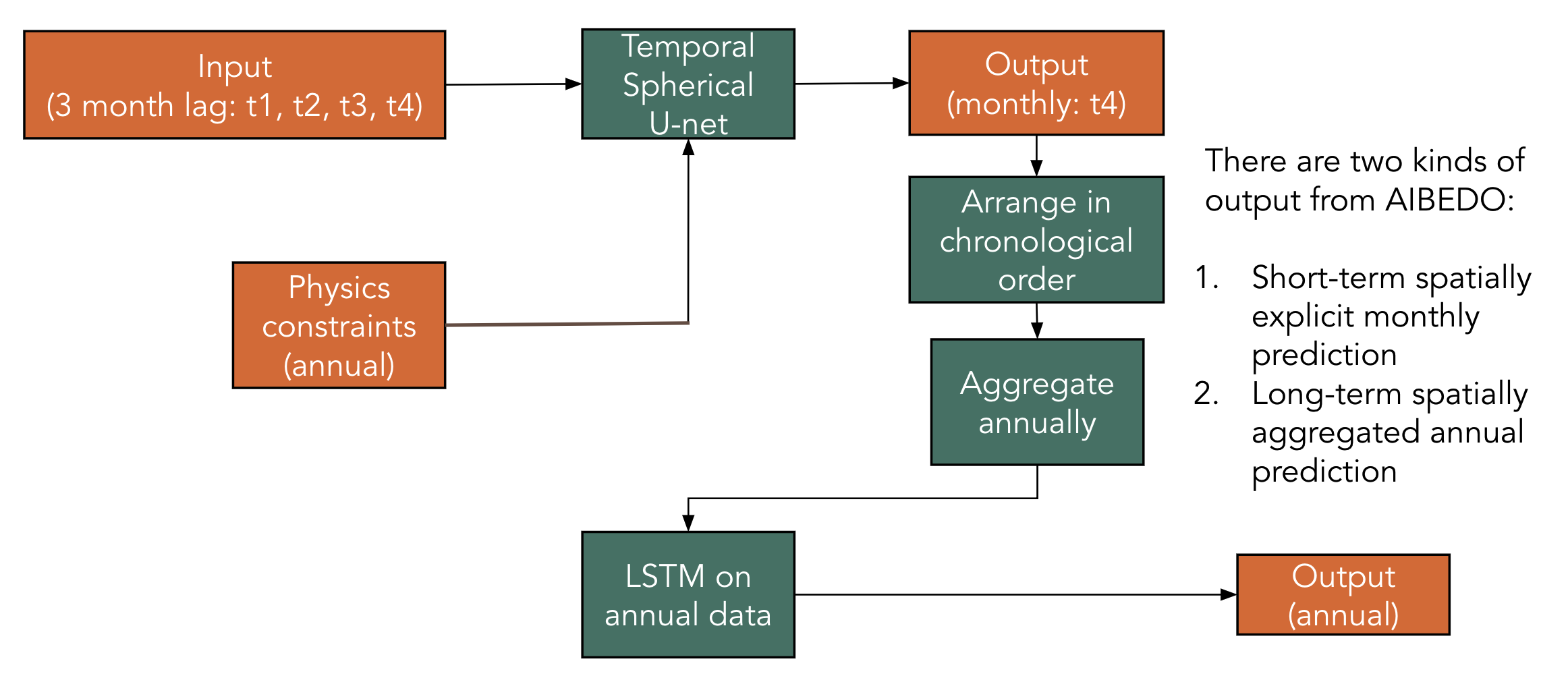
Figure 1. Schematic of AiBEDO Model Operation

Hybrid AI Model Architectures

MLP

A Multi-Layer Perceptron (MLP), also known as feedforward or fully connected network, is a simple neural network model. It operates on one-dimensional inputs and produces one-dimensional outputs. As in our case we have spatial data, it has to be flattened to a vector. That is, for spherical data of shape \((S, C_{in})\) we flatten it to a vector of size \(S * C_{in}\), where S is the number of spherical-pixels. Similarly, for 2D/euclidean data of shape \((H, W, C_{in})\) we flatten it to a vector of size \(H * W * C_{in}\), where H, W are the number of latitudes and longitudes.

class aibedo.models.MLP.AIBEDO_MLP(hidden_dims: Sequence[int], datamodule_config: Optional[omegaconf.dictconfig.DictConfig] = None, net_normalization: Optional[str] = None, activation_function: str = 'gelu', dropout: float = 0.0, residual: bool = False, residual_learnable_lam: bool = False, output_activation_function: Optional[Union[str, bool]] = None, *args, **kwargs)

Bases: aibedo.models.base_model.BaseModel

Multi-layer perceptron (MLP) AiBEDO model.

This model is agnostic to any spatial structure in the data, since it operates on 1D data vectors (spatial dimensions are flattened to 1D).

Parameters

• hidden_dims (List[int]) – The hidden dimensions of the MLP (e.g. [100, 100, 100])

• datamodule_config (DictConfig) – The config of the datamodule (e.g. produced by hydra <config>.yaml file parsing)

• net_normalization (str) – One of [‘batch_norm’, ‘layer_norm’, ‘none’]. Default: “none”

• activation_function (str) – The activation function of the MLP. Default: ‘gelu’

• dropout (float) – How much dropout to use in the MLP. Default: 0.0 (no dropout)

• residual (bool) – Whether to use residual connections in the MLP. Default: False

• residual_learnable_lam (bool) – Whether to use residual connections with learnable lambdas

• output_activation_function (str, bool, optional) – By default no output activation function is used (None). If a string is passed, is must be the name of the desired output activation (e.g. ‘softmax’) If True, the same activation function is used as defined by the arg activation_function.

forward(X: torch.Tensor) → torch.Tensor

Forward the input through the MLP.

Shapes:

• Input: \((B, *, C_{in})\)

• Output: \((B, *, C_{out})\),

where \(B\) is the batch size, \(*\) is the spatial dimension(s) of the data, and \(C_{in}\) (\(C_{out}\)) is the number of input (output) features. Internally are spatial dimensions are flattened together with \(C_{in}\) into a single dimension.

Spherical U-Net

U-net is a specific form of convolutional neural network (CNN) architecture that consists of pairs of downsampling and upsampling convolutional layers with pooling operations. Unlike regular CNNs, the upsampling feature channels help the model learn the global location and context simultaneously. This technique has been proven extremely useful for biomedical applications and recently has been adopted in the earth sciences. While this is a more effective technique, one of the limitations of U-net architecture when applied to earth sciences is the inability to capture the spherical topology of data. Typically they are resolved by including boundary layer conditions/constraints. In our approach, we adopt a variant of U-net called “spherical U-net” for modeling the spatial component of AIBEDO, which is a geodesy-aware architecture and hence accounts for the spherical topology of Earth System data alleviating the need for external architectural constraints.

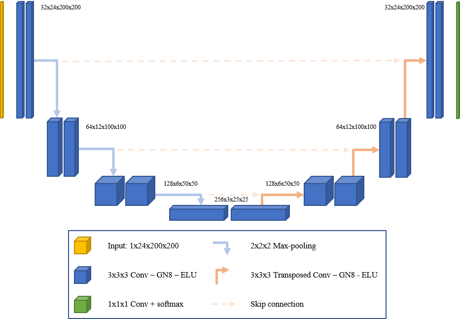
Figure 2. Schematic of U-net Architecture

The model uses special convolutional and pooling operations for representing spherical topology through Direct Neighbor (DiNe) convolution and spherical surface pooling operations. Also, the model takes input in the icosahedral surface for the better representation of the earth surface by resampling from the original 2-dimensional NetCDF grid data.

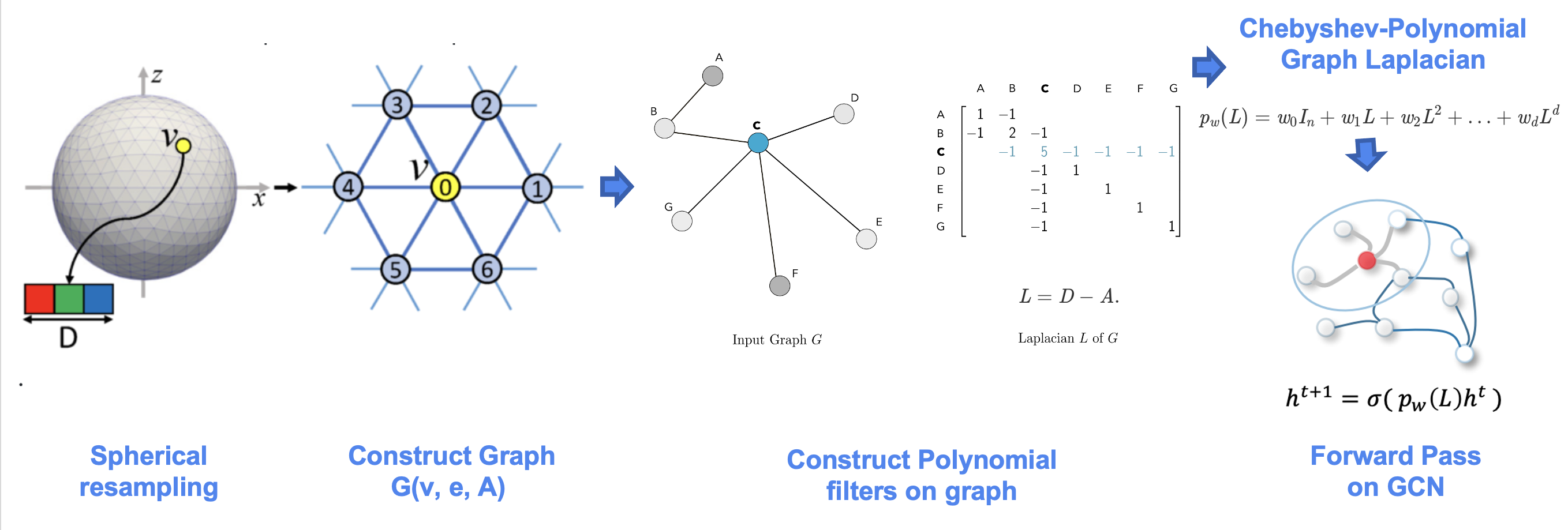
Figure 3. Spherical U-net Graph Convolution

Spherical Graph Convolutional Neural Network with UNet autoencoder architecture.

class aibedo.models.unet.SphericalUNet(pooling_class: str, depth: int, laplacian_type: str, kernel_size: int, ratio: float = 1.0, **kwargs)

Bases: aibedo.models.base_model.BaseModel

Spherical GCNN Autoencoder.

Parameters

• pooling_class (str) – One of three classes of pooling methods

• depth (int) – The depth of the UNet, which is bounded by the N and the type of pooling

• kernel_size (int) – chebychev polynomial degree

• ratio (float) – Parameter for equiangular sampling

forward(x: torch.Tensor)

Forward Pass.

Parameters

x (torch.Tensor) – input to be forwarded.

Returns

torch.Tensor – output

Training and Testing

The following are the main functions that you want to use for training and/or testing the AiBEDO models.

train.run_model	This function runs/trains/tests the model.
test.reload_and_test_model	This function reloads a model from a checkpoint and trains and/or tests it.

Interface

The main training and testing scripts above, calls various helper functions to avoid model/data loading (and reloading) boilerplate code. If the main training/testing scripts above are not enough for your purposes, we strongly recommend using the interface functions below as much as possible.

interface.get_model	Get the AIBEDO model, a subclass of BaseModel, as defined by the key value pairs in config.model.
interface.get_datamodule	Get the datamodule, as defined by the key value pairs in config.datamodule.
interface.get_model_and_data	Get the model and datamodule.
interface.reload_model_from_config_and_ckpt	Load a model as defined by config.model and reload its weights from model_path.