Tip

This tutorial is available as a Jupyter notebook.

Demo notebook

This notebook will show you how to use a trained AiBEDO model for inference. That is, we will reload the weights of a trained model to use it for predicting a single snapshot (time-step) of the data, as well as visualizing the corresponding predictions and errors.

Data requirements

To run this notebook you need to have the following data (in DATA_DIR directory, which is defined below):

• epoch023_seed15.ckpt - the checkpoint of the trained model

• compress.isosph.CESM2.historical.r1i1p1f1.Input.Exp8_fixed.nc - the input data for AiBEDO

• compress.isosph.CESM2.historical.r1i1p1f1.Output.PrecipCon.nc - the target/ground-truth data for reference

• ymonmean.1980_2010.compress.isosph.CMIP6.historical.ensmean.Output.PrecipCon.nc - Mean statistics for denormalization of predictions

• ymonstd.1980_2010.compress.isosph.CMIP6.historical.ensmean.Output.PrecipCon.nc - Std. statistics for denormalization of predictions

Note that you can use any other data for inference, e.g. from a different ESM or from reanalysis data (e.g. ERA5).

# Please define the path where the data and model checkpoint is stored
DATA_DIR = "../../data"

Setting up our workspace

Imports

In this section we’ll set up our workspace. We’ll import the necessary packages, and setup our data and model. First, the imports:

import os
# Make sure we're in the right directory
if os.path.basename(os.getcwd()) in ["examples", 'notebooks']:
    os.chdir("..")
import torch
import xarray as xr
import numpy as np
from typing import *
import cartopy.crs as ccrs
import matplotlib.pyplot as plt
from aibedo.models.base_model import BaseModel
from aibedo.models.MLP import AIBEDO_MLP
# from aibedo.models.unet import SphericalUNet

Paths and filenames

*Please edit here to your own paths and desired filenames*

# Input data filename (isosph is an order 6 icosahedron, isosph5 of order 5, etc.)
filename_input = "compress.isosph.CESM2.historical.r1i1p1f1.Input.Exp8_fixed.nc"
# Output data filename (inferred from the input filename), do not edit!
# E.g.: "compress.isosph.CESM2.historical.r1i1p1f1.Output.PrecipCon.nc"
filename_output = filename_input.replace("Input.Exp8_fixed", "Output.PrecipCon")
# Define the timestep to use as input data (as absolute index, -10 means 10 timesteps before the last timestep)
prediction_timestep = -10
# Define the ML model checkpoint path to be reloaded
CKPT = 'epoch023_seed15.ckpt'

Some constants that we will use later on (do not edit)

# _pre means that the variable has been pre-processed (i.e. deseasonalized, detrended, etc.)
VARS_INPUT = [ 'crelSurf_pre', 'crel_pre', 'cresSurf_pre', 'cres_pre', 'netTOAcs_pre', 'lsMask', 'netSurfcs_pre']
VARS_OUTPUT = ['tas', 'ps', 'pr']
output_var_clean_name = {
    'tas': 'Air Temperature',
    'ps': "Surface Pressure",
    'pr': "Precipitation",
}

Loading data and (re-)loading model

Now that we have defined all the paths and filenames, we can load the data and the model (and reload the model weights).

Load the pre-processed data

ds_input = xr.open_dataset(f"{DATA_DIR}/{filename_input}")  # Input data
ds_output = xr.open_dataset(f"{DATA_DIR}/{filename_output}") # Ground truth data
ds_input.crel_pre.values.shape  # (time, pixel-in-icosahedron)

(1980, 40962)

Load the model

# Get the appropriate device (GPU or CPU) to use
device = torch.device('cuda' if torch.cuda.is_available() else 'cpu')
# Load the trained model checkpoint (its weights, hyperparameters, etc.)
saved_model = torch.load(f"{DATA_DIR}/{CKPT}", map_location=device)
saved_model['hyper_parameters']['datamodule_config']['data_dir'] = DATA_DIR   # Update the data directory
# Get the appropriate architecture to use based on the hyperparameters
model = AIBEDO_MLP(**saved_model['hyper_parameters'], use_auxiliary_vars=False)
saved_model['hyper_parameters']

{'datamodule_config': {'_target_': 'aibedo.datamodules.icosahedron_dm.IcosahedronDatamodule', 'order': 6, 'time_lag': 0, 'partition': [0.85, 0.15, 'merra2'], 'data_dir': '../../data', 'input_filename': 'compress.isosph.CESM2.historical.r1i1p1f1.Input.Exp8_fixed.nc', 'input_vars': ['crelSurf_pre', 'crel_pre', 'cresSurf_pre', 'cres_pre', 'netTOAcs_pre', 'lsMask', 'netSurfcs_pre'], 'output_vars': ['tas_pre', 'ps_pre', 'pr_pre'], 'batch_size': 10, 'eval_batch_size': 30, 'num_workers': 2, 'pin_memory': True, 'verbose': True, 'seed': 43},
 'input_transform': {'_target_': 'aibedo.data_transforms.transforms.FlattenTransform'},
 'optimizer': {'name': 'adamw', 'lr': 0.0002, 'weight_decay': 1e-06, 'eps': 1e-08},
 'scheduler': {'_target_': 'torch.optim.lr_scheduler.ExponentialLR', 'gamma': 0.98},
 'monitor': 'val/mse',
 'mode': 'min',
 'window': 1,
 'loss_weights': [0.333, 0.333, 0.333],
 'physics_loss_weights': [0, 0, 0, 0, 0],
 'nonnegativity_at_train_time': True,
 'month_as_feature': False,
 'loss_function': 'mean_squared_error',
 'name': '',
 'verbose': True,
 'hidden_dims': [1024, 1024, 1024, 1024],
 'net_normalization': 'layer_norm',
 'activation_function': 'Gelu',
 'dropout': 0.0,
 'residual': True,
 'residual_learnable_lam': False,
 'output_activation_function': None}

Reload the checkpoint (model weights)

model.load_state_dict(saved_model['state_dict'])

<All keys matched successfully>

Pre-process the data to be used for the ML model

To input the loaded data into the model, we need to pre-process the .nc data. Here, we need to first concatenate all input variables to the feature/channel dimension.

def concat_variables_into_channel_dim(data: xr.Dataset, variables: List[str]) -> np.ndarray:
    """Concatenate xarray variables into numpy channel dimension (last)."""
    assert len(data[variables[0]].shape) == 1, "Each input data variable must have only one dimension"
    data_ml = np.concatenate(
        [data[var].values.reshape((-1, 1)) for var in variables],
        axis=-1  # last axis
    )
    return np.expand_dims(data_ml, axis=0).astype(np.float32)  # Add a batch dimension

Next, we also need to keep track of the month of the output data, since after inference we need to denormalize the raw predictions based on monthly statistics (so that they are in the original-scale, e.g. Kelvin for temperature).

def get_month_of_output_data(output_xarray: xr.Dataset) -> np.ndarray:
    """ Get month of the snapshot (0-11), needed for denormalization with monthly statistics.  """
    n_gridcells = len(output_xarray['ncells'])
    # .item() is required here as only one timestep is used, the subtraction with -1 because we want 0-indexed months
    month_of_snapshot = np.array(output_xarray.coords['time'].item().month, dtype=np.float32) - 1
    # now repeat the month for each grid cell/pixel
    dataset_month = np.repeat(month_of_snapshot, n_gridcells)
    return dataset_month.reshape([1, n_gridcells, 1])  # Add a batch dimension and dummy channel/feature dimension

With the following function, we glue functions methods above and also make the resulting data PyTorch ready, i.e. make it a torch.Tensor, move it to the correct device (CPU/GPU).

def get_pytorch_model_data(input_xarray: xr.Dataset, output_xarray: xr.Dataset, timestep_i: int) -> torch.Tensor:
    """Get the tensor input data for the ML model at the specified timestep."""
    snapshot_input_raw = input_xarray.isel(time=timestep_i)
    snapshot_output_raw = output_xarray.isel(time=timestep_i)
    # Concatenate all variables into the channel/feature dimension (last) of the input tensor
    data_input = concat_variables_into_channel_dim(snapshot_input_raw, VARS_INPUT)
    # Get the month of the snapshot (0-11), which is needed to denormalize the model predictions into their original scale
    data_month = get_month_of_output_data(snapshot_output_raw)
    # For convenience, we concatenate the month information to the input data, but it is *not* used by the model!
    data_input = np.concatenate([data_input, data_month], axis=-1)
    # Convert to torch tensor and move to CPU/GPU
    data_input = torch.from_numpy(data_input).float().to(device)
    return data_input

snapshot_input_ml = get_pytorch_model_data(ds_input, ds_output, prediction_timestep)
snapshot_target = ds_output.isel(time=prediction_timestep)
snapshot_input_ml.shape  # (batch-dimension, icosahedron-grid-dimension, feature-dimension)

torch.Size([1, 40962, 8])

Prediction with the AiBEDO model

*Note:* Please always use the model.predict(input_tensor) method instead of model(input_tensor)!!!

def predict_with_aibedo_model(aibedo_model: BaseModel, input_tensor: torch.Tensor) -> Dict[str, torch.Tensor]:
    """
    Predict with the AiBEDO model.
    Returns:
        A dictionary of output-variable -> prediction-tensor key->value pairs.
        Each prediction-tensor has been denormalized to original scale (e.g. temperature in kelvin)
    """
    model.eval()
    with torch.no_grad():  # No need to track the gradients during inference
        prediction = aibedo_model.predict(input_tensor)
    return prediction

snapshot_prediction = predict_with_aibedo_model(model, snapshot_input_ml)
snapshot_prediction.keys()

dict_keys(['tas', 'ps', 'pr'])

Post-processing and plotting

def get_predictions_xarray(targets_ds: xr.Dataset, predictions_ds: xr.Dataset) -> xr.Dataset:
    """ Add the torch tensor predictions to the xarray targets dataset as well as errors (bias, MAE). """
    return_ds = targets_ds.copy()
    for var, pred in predictions_ds.items():
        pred_key = f"{var}_pred"
        return_ds[pred_key] = ('ncells', pred.squeeze().cpu().numpy())
        # compute the error
        diff_err = return_ds[pred_key] - return_ds[var]
        return_ds[f'{var}_mae'] = np.abs(diff_err)
        return_ds[f'{var}_bias'] = diff_err
    return return_ds

snapshot_postprocessed = get_predictions_xarray(snapshot_target, snapshot_prediction)

A plotting script

def single_snapshot_plotting(postprocessed_xarray: xr.Dataset,
                       **kwargs
                       ):
    proj = ccrs.PlateCarree()
    plot_kwargs = dict(
        ds=postprocessed_xarray,
        x='lon',
        y='lat',
        transform=proj, subplot_kws={'projection': proj},
        cbar_kwargs={'shrink': 0.8,  # make cbar smaller/larger
                     'pad': 0.01,  # padding between right-most subplot and cbar
                     'fraction': 0.05}, **kwargs
    )
    nrows, ncols = 4, 3
    fig, axs = plt.subplots(nrows, ncols, sharex=True, sharey=True,
                            subplot_kw={'projection': proj},
                            gridspec_kw={'wspace': 0.07, 'hspace': 0,
                                         'top': 1., 'bottom': 0., 'left': 0., 'right': 1.},
                            figsize=(ncols * 12, nrows * 6)  # <- adjust figsize but keep ratio ncols/nrows
                            )

    for j, var in enumerate(VARS_OUTPUT):
        p_target = xr.plot.scatter(hue=var, ax=axs[0, j], **plot_kwargs)
        p_preds = xr.plot.scatter(hue=f'{var}_pred', ax=axs[1, j], vmin=p_target.colorbar.vmin, vmax=p_target.colorbar.vmax, **plot_kwargs)
        p_bias = xr.plot.scatter(hue=f'{var}_bias', ax=axs[2, j], **plot_kwargs)
        p_mae = xr.plot.scatter(hue=f'{var}_mae', ax=axs[3, j], **plot_kwargs)

        # Set title
        axs[0, j].set_title(output_var_clean_name[var], size=30)

        # Edit colorbar
        for p, label in zip([p_target, p_preds, p_bias, p_mae], ['Targets', "AiBEDO", 'Bias', "MAE"]):
            p.colorbar.set_label(label, size=25)
            p.colorbar.ax.tick_params(labelsize=18)

    for ax in list(axs.flat):
        ax.coastlines(linewidth=0.5)

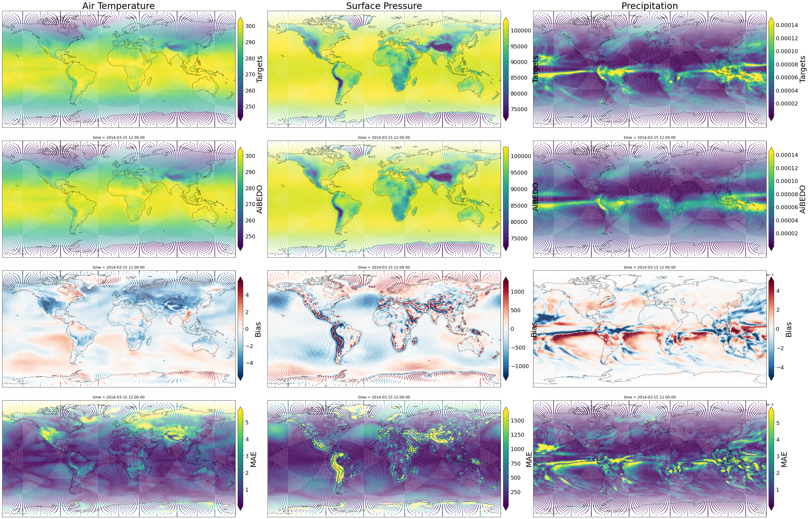
Plotting the results

Legend:

Each column is a different (denormalized) output variable.

Rows:
- First row: Targets
- Second row: AiBEDO model predictions
- Third row: Bias error (AiBEDO - Targets)
- Fourth row: MAE error (|AiBEDO - Targets|)

Note the 1e-5 in the precipitation errors!

single_snapshot_plotting(snapshot_postprocessed, robust=True, s=2)