Preprocessing and Spherical Grid

Detrend, Deseasonalize and Normalize

Our preprocessing code respository can be found here that consists of several scripts to preprocess various Earth System Model ensembles. For example, the following code block shows a simple method to preprocess CESM2-WACCM model ensemble:

import preprocessing

#activity = 'CMIP'
#experiment = 'historical'

activity = 'ScenarioMIP'
experiment = 'ssp585'
institute = 'NCAR'
modelName = 'CESM2-WACCM'

for member in ['r2i1p1f1','r3i1p1f1']:
    #member = 'r1i1p1f1'
    preprocessing.preprocess_input(activity, experiment, modelName, institute, member)
    preprocessing.preprocess_output(activity, experiment, modelName, institute, member)

Running this script preprocesses the model data to detrend, deseasonalize and normalize (detailed in Datasets section). We have provided similar high-level scripts for the selected ESM models we are using in our training data.

Interpolate 2D-gridded data to Spherical Grids

We use pygsp package to interpolate 2D-gridded data into a spherical grid format. This is done in two steps:

Step 1: Generate a text file (“skeleton”) with the desired Icosahedral level using our python script (link here). The code block is also shown below:

import pygsp as pg
import numpy as np

### Generates a text file with centre points of a icosahedral sphere grid
### Formatted to pass as an argument for 'cdo remap,GRIDFILE in.nc out.nc'

def xyz2lonlat(x:float,y:float,zLfloat, radius=6371.0e6):
    """From cartesian geocentric coordinates to 2D geographic coordinates."""
    """ lon: [-180, 180], lat:[-90, 90] """
    latitude = np.arcsin(z / radius)/np.pi*180
    longitude = np.arctan2(y, x)/np.pi*180
    return longitude, latitude

def gen_icosphere(level:int,radius:float = 6371.0e6):
    '''
    Generates points on a icosphere grid (from Soo Kim)
    level (int): iteration level
    radius (float): radius of the earth
    '''
    #(1) generate graph of SphereIcosahedral
    graph = pg.graphs.SphereIcosahedral(2**level)
    #(2) extract lon, lat coordinate
    vertices = graph.coords # xyz coordinates
    #print("number of vertices for level "+str(level)+" (2**"+str(level)+")is "+str(graph.n_vertices))
    lon = []
    lat = []
    radius = 1
    # convert cartesian points to spherical lon/lat
    for tmp_xyz in vertices:
        tmp_lon, tmp_lat = xyz2lonlat(tmp_xyz[0],tmp_xyz[1],tmp_xyz[2], radius=radius)
        lon.append(tmp_lon)
        lat.append(tmp_lat)
    return lon, lat

sphlevel = 6

lon,lat = gen_icosphere(sphlevel,radius = 6371.0e6)

f = open("isosphere_{0}.txt".format(sphlevel), "a")

# write grid to file
f.write("gridtype = unstructured\n")
f.write("gridsize = {0}\n".format(len(lon)))
f.write("# Longitudes\n")
f.write("xvals = " + ' '.join(map(str, lon))+"\n")
f.write("# Latitudes\n")
f.write("yvals = " + ' '.join(map(str, lat))+"\n")

This code block generates a text file that will be used to generate the spherical sample for level 6. To generate a text file for another grid level, please change the sphlevel in the code.

Step 2: Once the text file is generated in step 1, we use the cdo (Climate Data Operator) command line tool to generate the interpolated netCDF file. Please see here for instructions to download cdo.

The following script is given in command line to generate the interpolated file for model training:

cdo remapbil,icosphere_6.txt in.nc out.nc

Here, in.nc is the 2D-gridded file from ESM model ensembles or Reanalysis datasets, and out.nc is the name of the interpolated file that will be used for model training.

Sampling Module

Typically, models use climate data in a uniform 2D rectangular gridded pattern. While this may suffice local/regional modeling attributes, they do not capture the physical/geodesy properties of the Earth, particularly as the focus moves away from the equator. For this reason, we developed a geodesy-aware sampling that converts 2D rectangular gridded coordinates to a geodesic grid type. There are several ways a geodesic grid can be manifested. Our method allows the modeler to choose the target gridding type between two such mesh types: (a) Icosahedral, (b) Healpix.

Icosahedral Grids: Icosahedral grids consist of a certain number of equiangular triangles to form a convex polygon, called Icosahedron. The triangles are formed by equally spaced grid points to form a sphere. The number of grid points are defined by their levels as shown in the following equation:

Here, g refers to the grid level we want to generate the mesh for, and N refers to the number of points in the grid that forms the icosahedron.

Figure 3. Illustration of Icosahedral meshes for different levels

Table 1. Icosahedral Levels, Vertices and Spatial Resolution

Levels	Vertices	Resolution
1	42	3520 km
2	162	1760 km
3	642	880 km
4	2562	440 km
5	10242	220 km
6	40962	110 km

Healpix Grids: Healpix is a curvilinear partition grid type made up of equal area quadrilaterals. Unlike icosahedral grids, they are manifested as pixels, and the total number of pixels in a Healpix grid is calculated as follows:

Here P is the number of pixels in the Healpix grid, and S is the grid sub-division or resolution param- eter. Healpix is constructed in such a way that the areas of each pixel for a given sub-division is equal.

Figure 4. Illustration of Healpix meshes for different Subdivisions

Table 2. Healpix Subdivisions, Vertices and Spatial Resolution

Subdivisions	Vertices	Resolution
4	192	2497 km
8	768	1248 km
16	3072	6124 km
32	12288	312 km
64	49152	156 km
128	196608	78 km

Interpolation Module

We use the PyGSP library in Python to perform the grid transformation. It is commonly used for various graph operations to use in signal processing or social network analysis (e.g., Erdos-Reyni network). We first develop a ‘backbone’ structure of a spherical coordinate system (icosahedron, healpix, etc.). The properties of the spherical coordinates, such as levels or sub-divisions, are given as input. At this point, the coordinates are simply graph networks. In the next step, we assign latitude and longitude values to the graph network (x, y) so that they can be manifested in a geographical coordinate system. Finally, we use the raw data from reanalysis or ESM output and perform bilinear interpolation to obtain the final spherically-sampled data.

Figure 5. Pipeline to convert from 2D grid to Spherical grid

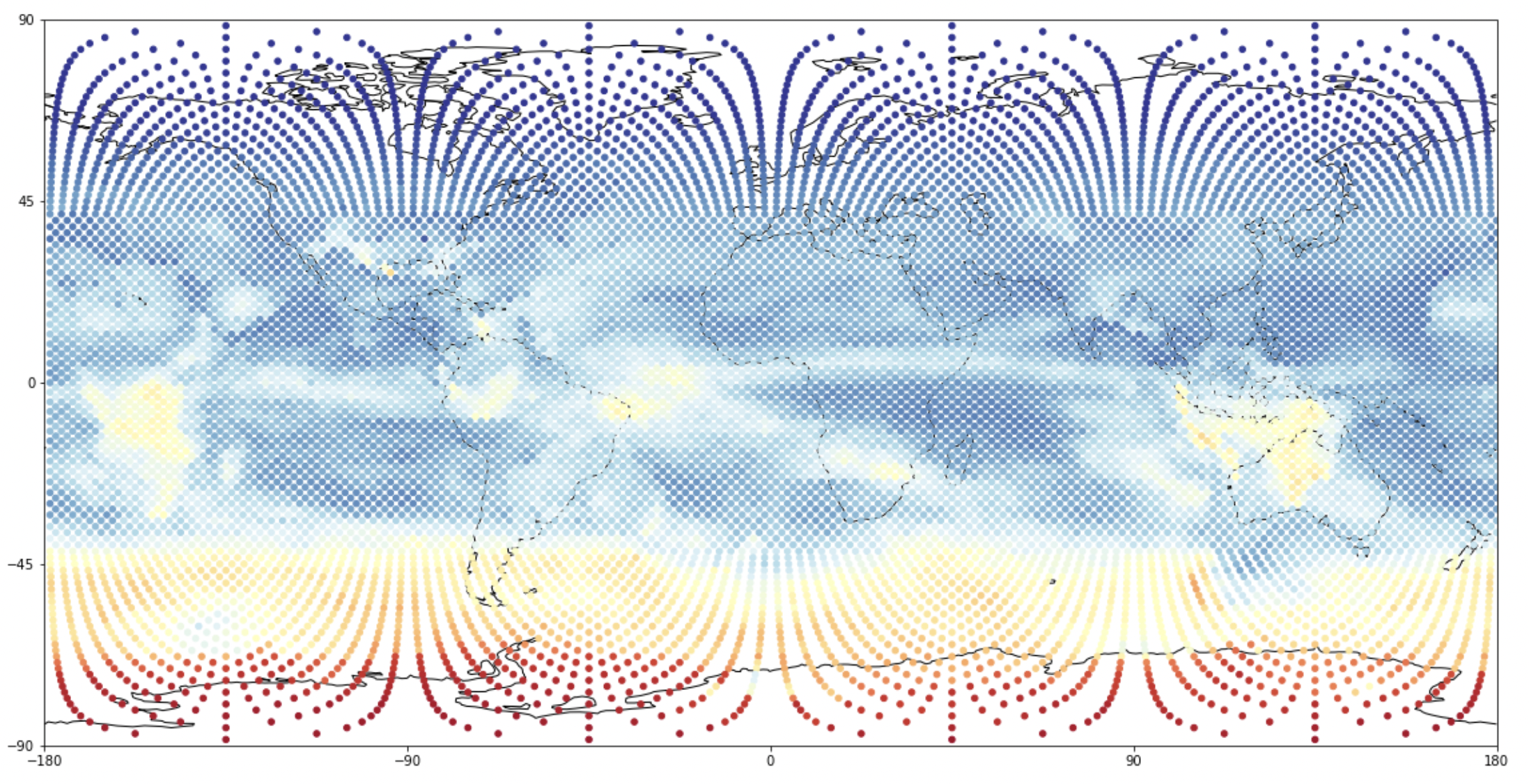
Figure 6. Spherical sampled and interpolated dataset from 2D-linearly gridded data