Datasets

Training data

Our training data for Phase 1 consists of

AiBEDO is trained on Earth System Model (ESM) output. In the case of the simultaneous model used for evaluating cloud-climate variability, we train on a subset of CMIP6 Earth System Model (ESM) outputs which had sufficient data availability on AWS to calculate the requisite input variables for our analysis (shown in Table 1. For each ESM, there are three categories of data hyper-cubes: (a) input, (b) output, and (c) data for enforcing physics constraints. Based on the initial results from our alpha hybrid model, we revised and increased the list of input variables to achieve better hybrid model performance. The updated list of input, output, and constraint variables is shown in Table 2. Furthermore, testing indicates that model performance improves when the model is trained on a large data pool from a single ESM, thus we have opted to train on long preindustrial control (piControl) simulations in addition to historical simulations.

Table 1. Earth System Model datasets for training simultaneous AiBEDO

Model	Historical (N)	piControl (years)	Lat spacing (deg)	Lon spacing (deg)
ACCESS-ESM1-5	0	900	1.25	1.875
AWI-ESM-1-1-LR	0	100	1.85	1.875
AWI-CM-1-1-MR	0	500	0.9272	0.9375
CESM2	1	1200	0.942	1.2500
CESM2-FV2	1	500	1.895	2.5000
CESM2-WACCM	1	499	0.942	1.2500
CESM2-WACCM-FV2	1	500	1.895	2.5000
CMCC-CM2-SR5	1	0	0.942	1.2500
CNRM-CM6-1-HR	0	100	0.495	0.5
CanESM5	5	1000	2.789	2.8125
E3SM-1-0	1	500	1.000	1.0000
E3SM-1-0	1	500	1.000	1.0000
EC-Earth3-Veg	0	500	0.695870	0.703125
GFDL-CM4	1	500	1.000	1.2500
GFDL-ESM4	1	500	1.000	1.2500
GISS-E2-1-H	1	401	2.000	2.5000
MIROC-ES2L	3	0	2.789	2.8125
MIROC6	1	0	1.400	1.4062
MPI-ESM-1-2-HAM	1	0	1.865	1.8750
MPI-ESM1-2-HR	1	0	0.935	0.9375
MPI-ESM1-2-LR	1	1000	1.865	1.8750
MRI-ESM2-0	1	0	1.121	1.1250
NorCPM1	5	0	1.9	2.5
SAM0-UNICON	1	0	0.942	1.2500

Table 2. Variable list and descriptions

Category	Variable	Description	Equation notation
Input	cres	TOA Cloud radiative effect in shortwave (positive down)	\(R_{TOA}^{cl,SW}\)
Input	cresSurf	Surface Cloud radiative effect in shortwave (positive down)	\(R_{SRF}^{cl,SW}\)
Input	crel	TOA Cloud radiative effect in longwave (positive down)	\(R_{TOA}^{cl,LW}\)
Input	crelSurf	Surface Cloud radiative effect in longwave (positive down)	\(R_{SRF}^{cl,LW}\)
Input	netTOAcs	TOA radiation without clouds (clear-sky) (positive down)	\(R_{TOA}^{cs,ALL}\)
Input	netSurfcs	Net Clearsky Surface radiation and heat flux (positive down)	\(R_{SRF}^{cs,ALL} - SH - LH\)
Output	tas	2-metre air temperature	\(T_{SRF}\)
Output	ps	Surface pressure	\(p_{SRF}\)
Output	pr	Precipitation	\(P\)
Constraint	evspsbl	Evaporation	\(E\)
Constraint	hfss	Surface upward sensible heat flux (positive up)	\(SH\)
Constraint	netTOARad	TOA All-sky radiation (positive down)	\(R_{TOA}^{all,ALL}\)
Constraint	netSurfRad	Surface All-sky radiation (positive down)	\(R_{TOA}^{all,ALL}\)
Constraint	qtot	Column integrated water vapour mass	\(Q_{tot} = \frac{1}{g}\sum_{lev} Q dp\)
Constraint	dqdt	Time tendency of column integrated water vapour mass	\(\frac{dQ_{tot}}{dt} = \frac{1}{g}\frac{d}{dt} \sum_{lev} Q dp\)

The ESM data are pooled together to form the training and testing datasets for our hybrid model. However, it is important to note there are substantial differences in the climatologies and variability of some of the chosen input variables across models. In particular, global average cloud liquid water content, cloud ice water content, and net top of atmosphere radiation vary more across ESMs than other variables. The former two are the result of differences in cloud parameterizations between ESMs, while the latter is likely due to uncertainties in the overall magnitude of anthropogenic forcing over the historical period. Comparing spatial correlation scores, shows net TOA radiation fields are very similar across models while the spatial pattern of cloud ice and water content varies substantially. Such variations represent the inter-ESM uncertainty in the representation of the climate. However, many of these ESM differences are largely removed during preprocessing described below.

When training a lagged model for MCB projections, we found we require a much larger, consistent sample of internal variability to train on. That is, we found that multi-model ensemble members of no-normalized data resulted errors in AiBEDO. Thus, we instead use data from the Community Earth System Model 2 (CESM2) Large Ensemble (LE) (Rodgers et al., 2021, Fig. 1), from which we use a 50-member ensemble of historical and SSP3-7.0 simulations with smoothed biomass burning. These are processed in the same manner as the CMIP6 data.

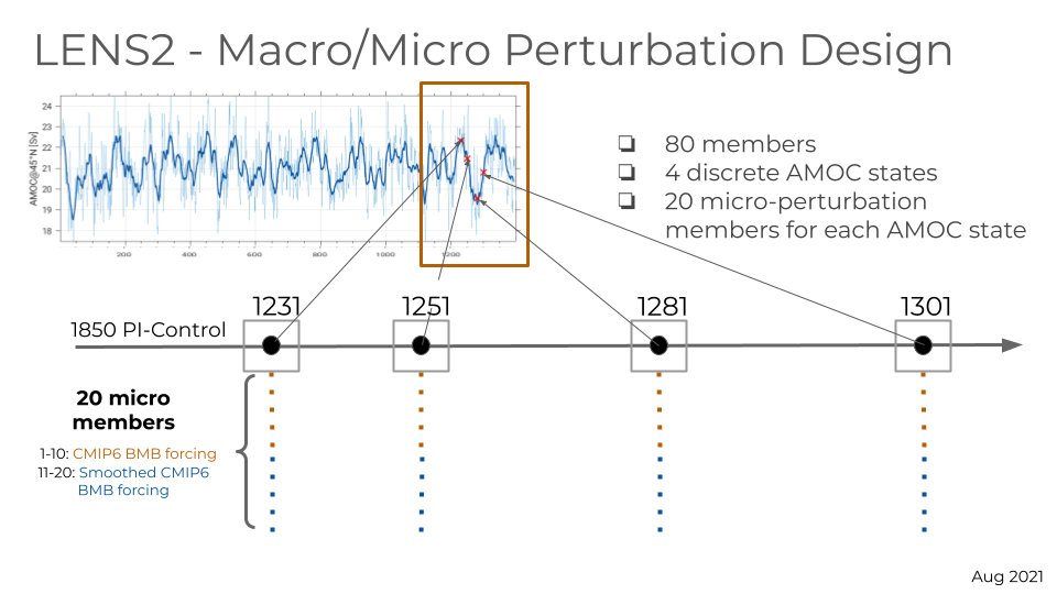
Figure 1. Initialization of CESM2 Large Ensemble simulations.

Reanalysis

In addition to ESM data, we also employ “reanalysis” datasets as validation datasets. Namely the Modern-Era Retrospective analysis for Research and Applications, Version 2 (MERRA2) and the ECMWF Reanalysis version 5 (ERA5). Reanalyses are models which ingest large quantities observational data to estimate the historical evolution of the atmosphere, thus providing an estimate of a wide range of atmospheric variables over the entire globe. While these data are not exactly the same as observational data, they are the best method of obtaining physically consistent and spatially complete climate data representing the recent past of the Earth’s atmosphere. MERRA2 includes data from 1980 to 2020 at 0.5 degree resolution and ERA5 includes data from 1979 to 2021 at 0.25 degree resolution.

Preprocessing

Each of the above data hyper-cubes are preprocessed before ingestion into the hybrid model. After testing with normalized and non-normalized training data, we find that the model produces better results when the variables are not normalized (i.e. not divided by the standard deviation at each grid points). Thus, our updated preprocessing pipeline is:

1. Remove seasonal cycle or “Deseasonalizing”: Subtract climatological seasonal cycle.

2. Remove trend or Detrend: Fit a third degree polynomial for each month of the year and subtract it from the data to remove trend in data over time. This removes secular trends (for example, rising temperatures as atmospheric CO$_2$ increases) and allows the model to be trained on fluctuations due to internal variability, rather than the forced response.

3. Remove rolling average: The anomaly at each grid point is calculated relative to a running mean that is computed over a centered 30-year window for that grid point and month.

4. Convert output variable units: Convert output variable units such that the magnitudes of the variables are similar

5. Remap data to Sphere-Icosahedral: Use Climate Data Operators to bilinearly remap different ESM grids to uniform level-5 or level-6 Sphere-Icosahedral grid.

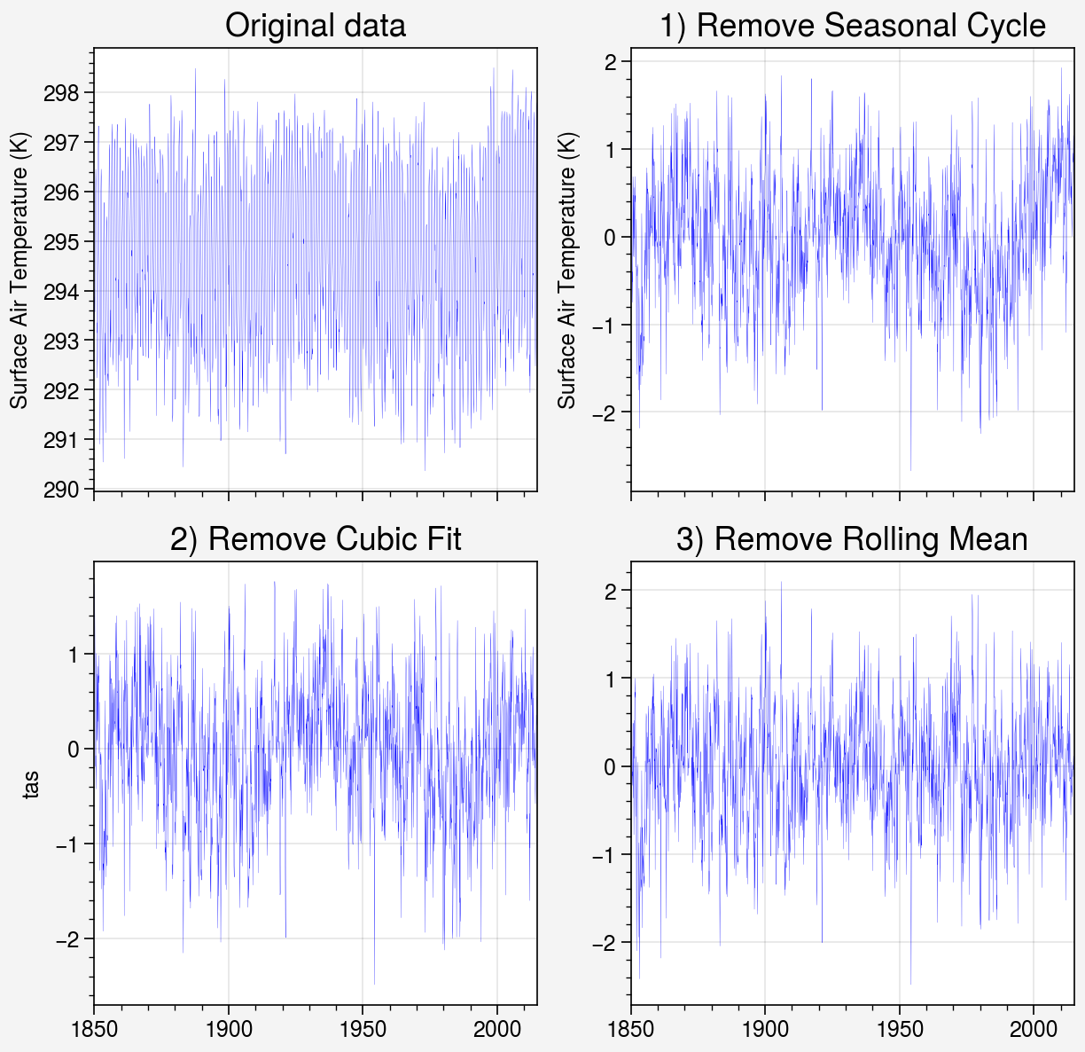
Figure 2. Example preprocessing for a surface air temperature data point.